Monetization: Two-Sided Network Simulation

Optional – Demand Curves
Here, we describe a single independent demand curve. You should understand this in order to understand coupled demand curves for the simulation in the next section. If you have had economics, feel free to skip or skim this section.
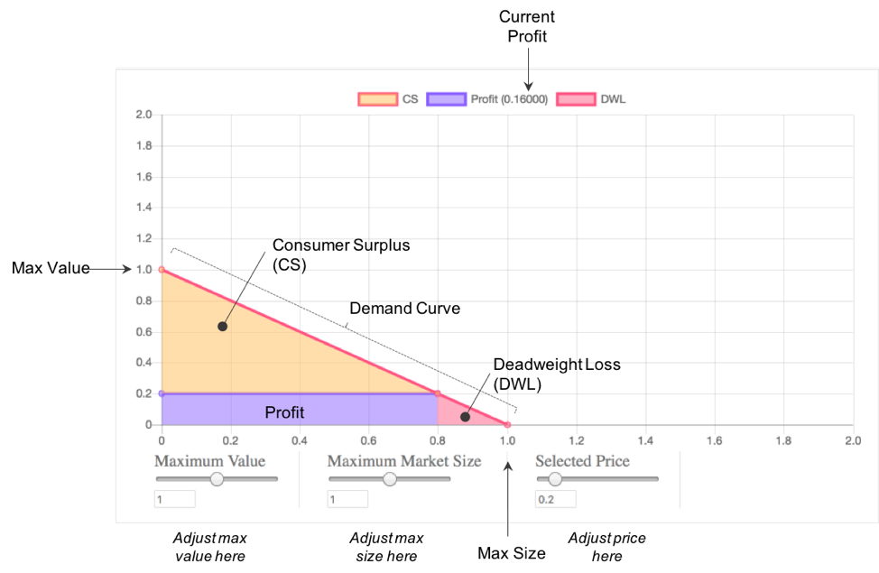
A demand curve represents graphically how much consumers will buy at a given price. The lower the price, the more they will buy. But, the lower the price, the lower is the profit per unit sold. The highest profit then balances competing pressures of trying to boost sales and trying to boost price. Everything is depicted in the figure below.

In the simulation below, you will be able to play with all the parameters shown here. In real life, the easiest thing to change is price. Normally, a company has great difficulty changing the maximum that consumers will pay for its product unless it changes the product. And a company has great difficulty changing the maximum size of the market, unless it finds a whole new market. The key concepts are the following:

Profit: This is just (Price) x (Quantity).  In the picture above, price = .2 and quantity = .8 so profit is (.2)(.8)=.16.  Units could be tens of thousands or millions, etc so .16 in profit would be $1,600 or $160,000 etc.. In this example, we’ve allowed marginal cost to be 0.  This is pretty accurate for information goods such as tweets and Facebook posts.  It’s also true for many platforms like Airbnb and Uber, where the firm does not incur the cost of a stay or a ride.  If you want to add costs, just calculate Profit = (Price – Cost) x (Quantity). Profit is the purple region of the plot.

Consumer Surplus: This represents the value of the purchase to the consumer beyond what the consumer paid.  Imagine you find a garment in your favorite store that has exactly the right fit and has great style.  Before you check the price, you decide it’s great but you won’t pay more than $120.  When you check the price, you find the store is charging $200.  The clerk just won’t negotiate so you walk away.  Two weeks later, the garment is on sale for half price so you buy it.  Your “surplus” is $20 since you would have paid $120 but, in the end, only paid $100. CS is the gold region of the plot.

Deadweight Loss: This is a fancy economic term for profitable sales that could have happened but didn’t. It’s a specific kind of opportunity cost.  In this region of the graph, there are consumers who would be willing to pay more than the firm’s cost to produce the good but less than the price the firm is currently charging. So why doesn’t the firm just charge less?  The firm could lower price but then it would earn less from all the current customers who do pay the current price.  Often a firm will try to capture this region by charging a high price initially then having a sale later but if consumers know this, they may choose to wait. DWL is the red region of the plot.

Simulation 1 – Explore a Demand Curve

Before you change end points of the demand curve (max value or max size), see if you can adjust price to maximize profits. The maximum you can achieve is (.25).

After maximizing profit, feel free to adjust the maximum value of the product i.e. consumers’ maximum willingness to pay, and also the maximum market size (i.e. how many consumers are in the market). Then try to optimize profit again after changing the market’s size and value. Now, maximum profit will depend on your specific choice of parameters.
As a rule, the maximum profit is equivalent to maximizing the area of the purple rectangle bounded by the red line of the demand curve. Interestingly, the shape of the demand curve really does not matter so long as it slopes down (i.e. people pay less as price rises). The demand curve can even be an arc that is bowed inward or outward and profits are still maximized by the largest rectangle that you can fit underneath.
The story above is the standard economic model for an independent good.

Simulation 2 – Explore an Interdependent Demand Curve Separately

The problem with the standard economic story is that it does not work for most platform goods that must get two (or more) sides on board. Demand curves for different groups can be interdependent. A pub might charge separate admission to men and to women, who attract one another. An operating system company might sell apps to consumers and system development kits (SDKs) to developers. They also attract one another.
The question is: what happens when we maximize profits on each individual product? In effect, this is what Steve Jobs did when he sold high priced Macs to consumers and he also sold high priced SDKs to developers.
In the simulation below, you’ve been put in charge of selling computers. Your job is to set price in order to maximize profits of your division. Steve Jobs has kept control of the developer division. You don’t get to set developer prices; he does.
Each of you will maximize profits in your respective division. You sell to consumers. Steve sells to developers.

Step 1: Choose consumer price to maximize division profits in your purple box.

Step 2: Click “Optimize Price for Developers” to tell Steve you’re done and let him optimize developer price.

Step 3: Repeat Steps 1 & 2 until your division profits are as high as you can make them. Run as many simulations as you like.

Step 4: When you have done as well as you can, record your best simulation run. Write down all three profits: for your division (purple box, consumer panel), for Steve’s division (orange box, developer panel) and for the whole company (white box total profit, in between panels). Write down also the prices and sales. To record sales, just estimate using the horizontal axis.  Estimate Steve’s price using the vertical developer axis.  Approximations are fine.

For your own purposes, create a simple table with all the following entries filled in.  You will report only cells with check marks. You will capture the exact same information for Sim-3 (another row) in a moment.

	Consumer Price	Cons. Sales	Cons. Profit	Developer Price	Dev. Sales	Dev. Profit	Total Profit
Sim-2			✓			✓	✓

 

Now ask yourself is this the best that the whole company can do?  What could you do differently?

Simulation 3 – Explore an Interdependent Demand Curve Collectively

Given your success with the computer division, Steve Jobs has put you in charge of pricing both divisions while he goes off and invents the iPod. Now you can control prices for consumers and for developers.

Step 1: Choose consumer price (left panel) to maximize profits in the total profit white box.

Step 2: Choose developer price (right panel) to maximize profits in the total profit white box.

Step 3: Repeat Steps 1 & 2 until your total firm profits are as high as you can make them.

Step 4: When you have done as well as you can, record your best simulation run. Write down all three profits: for the consumer division (purple box, consumer panel), for the developer division (orange box, developer panel) and for the whole company (white box total profit, in between panels). Write down also the prices and sales. To record sales, just estimate using the horizontal axis. Approximations are fine.

For your own purposes, complete the earlier table with all the following entries filled in.  Report only cells with check marks.

 

	Consumer Price	Cons. Sales	Cons. Profit	Developer Price	Dev. Sales	Dev. Profit	Total Profit
Sim-2			✓			✓	✓
Sim-3			✓			✓	✓

 

If you did this correctly, you should be able to achieve at least a 15% improvement in total profit by controlling both prices simultaneously.

When you are finished, post just the profit columns in the discussion forum with labels. Include the Sim-2 and Sim-3 information. DO NOT POST YOUR PRICES (THIS WOULD GIVE AWAY THE ANSWERS).

Simulation – Summary

Why should Sim-3 results be better than Sim-2 results? Wasn’t each division already as profitable as it could be? The answer is that the highest total profit for the entire firm is not the same as the sum of the highest total profit across the separate divisions. To see this, note that profits in the developer division for your Sim-3 are lower than the profits Steve Jobs achieved.  If Steve only looked at your profits in the developer division compared to what he achieved, he’d be pretty angry at you.

But your profit gains in the consumer division are now so much greater than your profit losses in the developer division, that dropping the price of SDKs in the developer market was totally worth it.

Because these markets experience a network effect, the prices and market sizes are interdependent.  More developers attract more consumers who attract more developers who attract more consumers, etc.. The market sizes are not fixed but are in fact co-determined. Participation on the same-side of the market affects participation on the cross-side of the market, and vice versa – the simulation accounts for this feedback. Now you can attract more developers by lowering their price, or possibly even subsidizing them.  This will bring in more consumers.

The optimal prices can go up or down for either side depending on the size and direction of the network effects. In this simulation, there are two network effects: (a) developers attract consumers, and (b) consumers attract developers. Here, developers are the stronger magnet so their price falls relative to the optimal independent price.  From your table, see how developer price dropped from Sim-2 to Sim-3. By contrast, optimal consumer price actually rose from Sim-2 to Sim-3 and yet sales also increased, despite your price hike.

This cannot happen for a standard independent good. In the context of network effects, however, the reason consumer sales can rise even when consumer prices also rise is that developer prices have fallen. With more developers using the SDKs, consumers are willing to pay more for the extra value developers have brought to the market. This interdependence is why normal pricing methods fail.

Note, both demand curves still slope downward. A price hike to consumers still causes a sales drop among consumers. Likewise, a price hike to developers still causes a sales drop among developers.  Rather the issue is that a price drop to developers can lead to a cross-side price hike among consumers (and vice versa). We must understand both same-side and cross-side effects of price shifts.

Here we introduce a bit of terminology.  The side of the market getting the price drop is the “subsidy side” and the side of the market getting the price hike is the “money side.”

The interdependence of prices is what makes pricing platforms so complex.  The more sides there are, the more complex the interdependencies.  As a rule, drop prices for that group that adds the most value or represents the strongest magnet.

 

For a deeper understanding of these issues, please see:

1. Parker, G. G., & Van Alstyne, M. W. (2005). Two-sided network effects: A theory of information product design. Management science, 51(10), 1494-1504. [for academics]
2. Eisenmann, T., Parker, G., & Van Alstyne, M. W. (2006). Strategies for two-sided markets. Harvard business review, 84(10), 92. [for practitioners]
3. Parker, G. G., & Van Alstyne, M. W. (2000). Information Complements, Substitutes & Strategic Product Design. Proceedings of the Twenty-First International Conference on Information Systems, 12(10), pp. 13-15. [for academics – first ever paper on two-sided markets]